K-NN 算法

K-NN(K-Nearest Neighbors) 算法也是用来分类的，他直观上十分容易理解：

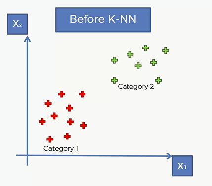
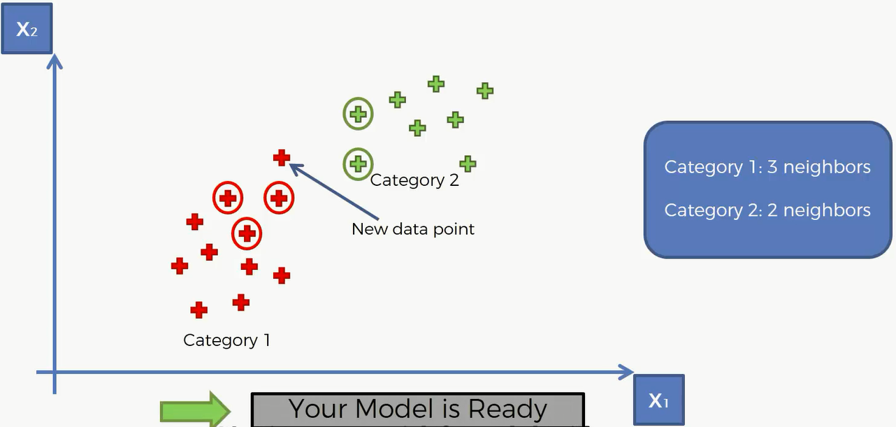
现在有两类，分别用红色的加号和绿色的加号描出，现在我们进来了一个新的数据点，我们的目标就是将这个数据点划到哪一类里面去。

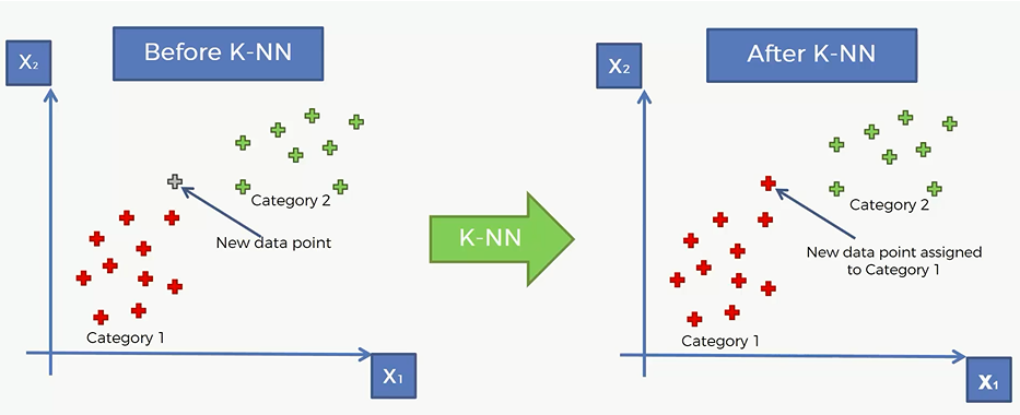
比如说下面这个点经过类K-NN 算法，被划归到红色的那一类取了

那么K-NN 算法是怎么运作的呢？ 其实很简单

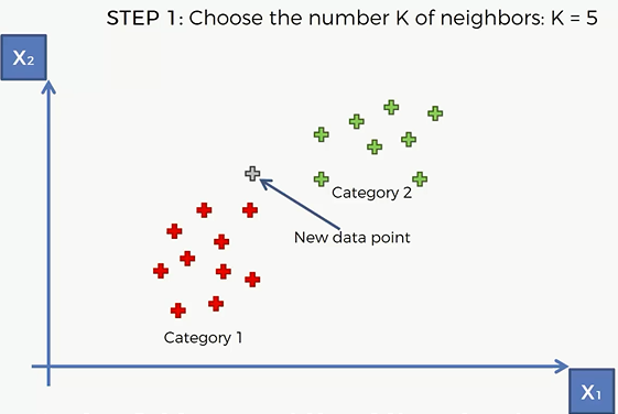
1. STEP1: Choose the number K of neighbors
2. STEP2: Take the K nearest neighbors of the new data point , according to the Euclidean distance
3. STEP3: Among these K neighbors ,count the number of data points in each category
4. STEP4: Assign the new data point to the category where you counted the most neighbors

结合上面这个写步骤，我们对刚才的例子进行剖析：

我们现决定要选取5个距离这个点最近的邻居

然后计算他和邻居之间的 Euclidean 距离，欧几里得距离的计算公式： $d=\sqrt{(x_2-x_1)^2+(y_2-y_1)^2}$

然后计算距离这个点最近5个欧几里得距离。在这5个最近的邻居中，属于红色区域的有3个，属于绿色区域的有2个，那么这个点就会被划分到红色区域当中去。

代码

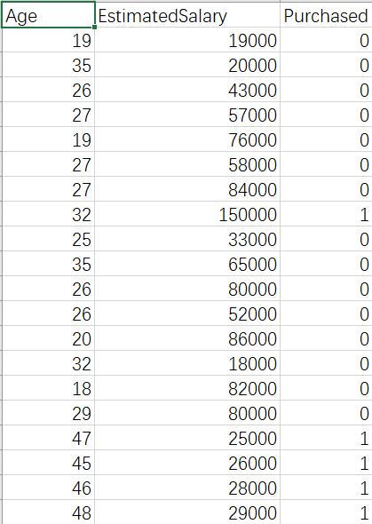
我们使用的数据集：

和逻辑回归的思路是一样的，只是换一个模型而已，所以这里略去重复的代码

Training the K-NN model on the Training set

n_neighbors =5 比较常用当然也可以多试试别的值来取最高的准确率

metric = ‘minkowski’ (闵可夫斯基) 就是说距离计算公式运用闵氏距离，是欧氏空间中的一种测度，被看做是欧氏距离和曼哈顿距离的一种推广。 $(\sum_{i=1}^n |x_i-y_i|^p)^{\frac{1}{p}}$

p=2就是 上面这个公式的 p

from sklearn.neighbors import KNeighborsClassifier
classifier = KNeighborsClassifier(n_neighbors = 5, 
                                  metric = 'minkowski', 
                                  p = 2)
classifier.fit(X_train, y_train)

看一下这个模型的混淆矩阵和准确分数：

from sklearn.metrics import confusion_matrix, accuracy_score
cm = confusion_matrix(y_test, y_pred)
print(cm)
accuracy_score(y_test, y_pred)

混淆矩阵：

[[64 4]
[ 3 29]]
准确度：0.93

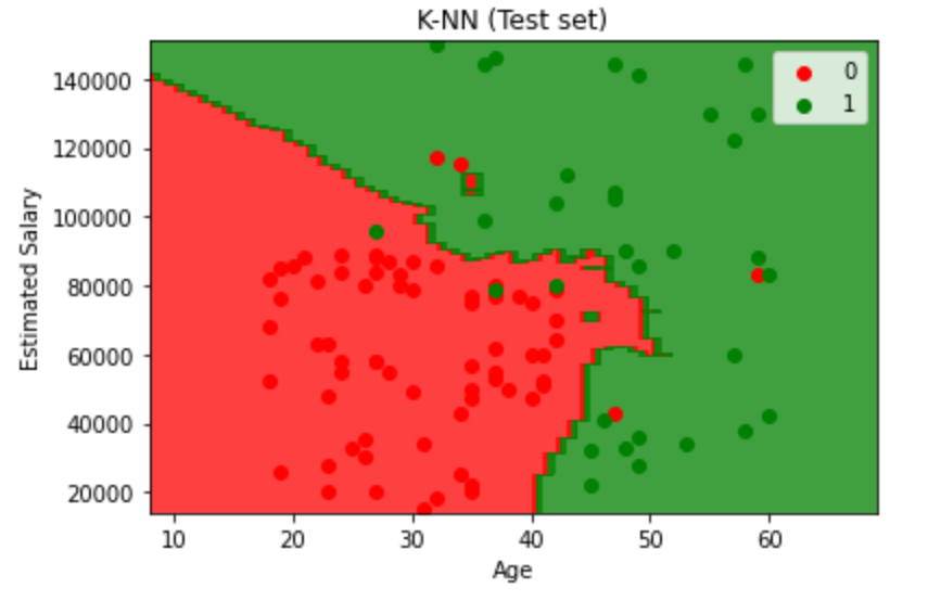
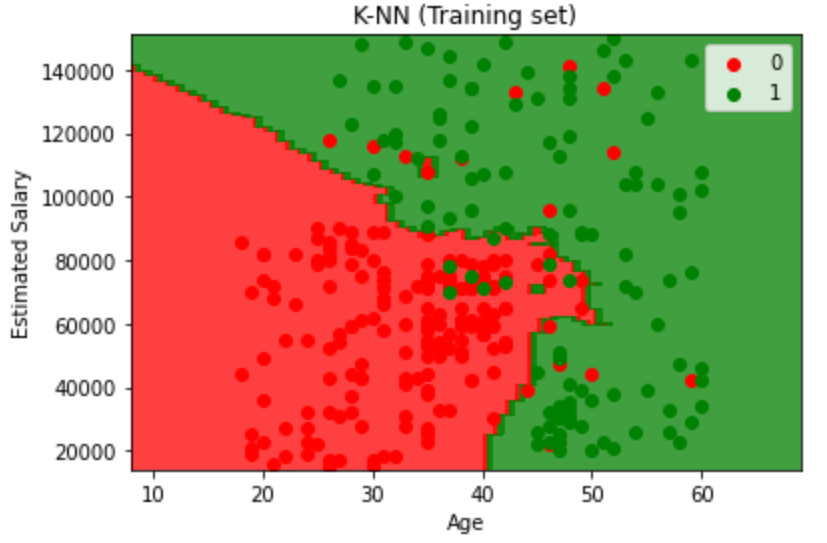
Visualising the Training set results

最后用可视化图来看一下结果：

from matplotlib.colors import ListedColormap
X_set, y_set = sc.inverse_transform(X_train), y_train
X1, X2 = np.meshgrid(np.arange(start = X_set[:, 0].min() - 10, stop = X_set[:, 0].max() + 10, step = 1),
                     np.arange(start = X_set[:, 1].min() - 1000, stop = X_set[:, 1].max() + 1000, step = 1))
plt.contourf(X1, X2, classifier.predict(sc.transform(np.array([X1.ravel(), X2.ravel()]).T)).reshape(X1.shape),
             alpha = 0.75, cmap = ListedColormap(('red', 'green')))
plt.xlim(X1.min(), X1.max())
plt.ylim(X2.min(), X2.max())
for i, j in enumerate(np.unique(y_set)):
    plt.scatter(X_set[y_set == j, 0], X_set[y_set == j, 1], c = ListedColormap(('red', 'green'))(i), label = j)
plt.title('K-NN (Training set)')
plt.xlabel('Age')
plt.ylabel('Estimated Salary')
plt.legend()
plt.show()

from matplotlib.colors import ListedColormap
X_set, y_set = sc.inverse_transform(X_test), y_test
X1, X2 = np.meshgrid(np.arange(start = X_set[:, 0].min() - 10, stop = X_set[:, 0].max() + 10, step = 1),
                     np.arange(start = X_set[:, 1].min() - 1000, stop = X_set[:, 1].max() + 1000, step = 1))
plt.contourf(X1, X2, classifier.predict(sc.transform(np.array([X1.ravel(), X2.ravel()]).T)).reshape(X1.shape),
             alpha = 0.75, cmap = ListedColormap(('red', 'green')))
plt.xlim(X1.min(), X1.max())
plt.ylim(X2.min(), X2.max())
for i, j in enumerate(np.unique(y_set)):
    plt.scatter(X_set[y_set == j, 0], X_set[y_set == j, 1], c = ListedColormap(('red', 'green'))(i), label = j)
plt.title('K-NN (Test set)')
plt.xlabel('Age')
plt.ylabel('Estimated Salary')
plt.legend()
plt.show()