决策树和随机森林分类器

决策树

在之前，我们介绍了回归树和随机森林回归现在我们来看看分类树

分类树和和回归树不同，它处理的数据都是离散的，且有分类的, 对于一个新数据的预测，我们是将其划归为哪一类中去。而回归树处理的数据则是连续的数字，对于一个新数据的预测，我们是赋给它一个值。

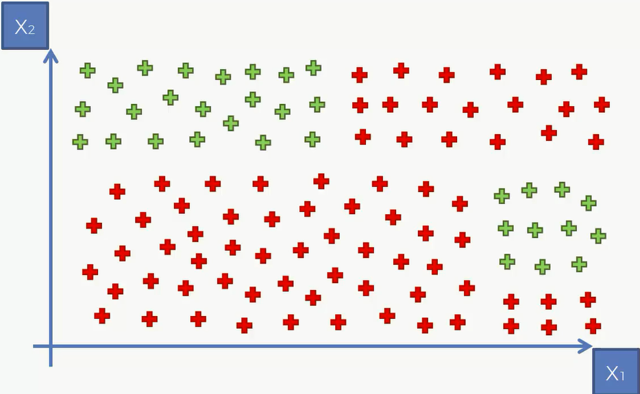
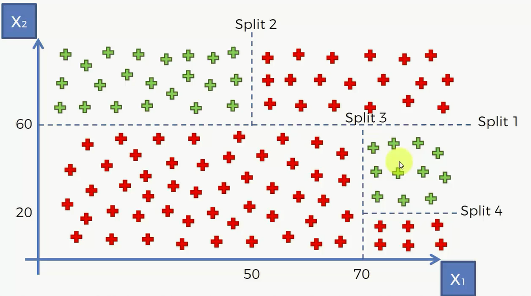
比如说下面这个例子，用分类树将其划分为几个区：

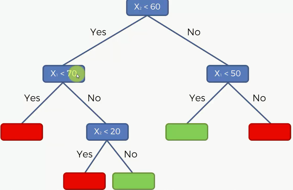
然后再对其进行决策：

决策树和其他的分类器一样，也可以对多个维度进行训练。

代码

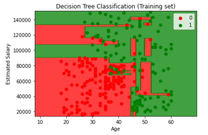
我们同样使用之前的年龄-薪资-购买与否的数据集：

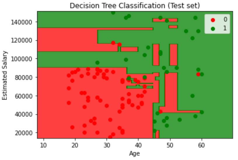
和之前的代码几乎一样，这里展示一下训练集、混淆矩阵以及可视化结果

Training the Decision Tree Classification model on the Training set

1
2
3

from sklearn.tree import DecisionTreeClassifier
classifier = DecisionTreeClassifier(criterion = 'entropy', random_state = 0)
classifier.fit(X_train, y_train)

Making the Confusion Matrix

from sklearn.metrics import confusion_matrix, accuracy_score
cm = confusion_matrix(y_test, y_pred)
print(cm)
accuracy_score(y_test, y_pred)

1
2
3

[[62  6]
 [ 3 29]]
 0.91

Visualizing the Training set results

from matplotlib.colors import ListedColormap
X_set, y_set = sc.inverse_transform(X_train), y_train
X1, X2 = np.meshgrid(np.arange(start = X_set[:, 0].min() - 10, 
							   stop = X_set[:, 0].max() + 10,
                               step = 0.25),
                     np.arange(start = X_set[:, 1].min() - 1000, 
                     			stop = X_set[:, 1].max() + 1000, 
                     			step = 0.25))
plt.contourf(X1, X2, 
classifier.predict(sc.transform(np.array([X1.ravel(), X2.ravel()]).T)).reshape(X1.shape),
             alpha = 0.75,
             cmap = ListedColormap(('red', 'green')))
plt.xlim(X1.min(), X1.max())
plt.ylim(X2.min(), X2.max())
for i, j in enumerate(np.unique(y_set)):
    plt.scatter(X_set[y_set == j, 0],
    			X_set[y_set == j, 1],
                c = ListedColormap(('red', 'green'))(i),
                label = j)
plt.title('Decision Tree Classification (Training set)')
plt.xlabel('Age')
plt.ylabel('Estimated Salary')
plt.legend()
plt.show()

from matplotlib.colors import ListedColormap
X_set, y_set = sc.inverse_transform(X_test), y_test
X1, X2 = np.meshgrid(np.arange(start = X_set[:, 0].min() - 10,
								stop = X_set[:, 0].max() + 10,
                                step = 0.25),
                     np.arange(start = X_set[:, 1].min() - 1000, 
                     			stop = X_set[:, 1].max() + 1000,
                                step = 0.25))
plt.contourf(X1, X2, 
classifier.predict(sc.transform(np.array([X1.ravel(), X2.ravel()]).T)).reshape(X1.shape),
             alpha = 0.75, 
             cmap = ListedColormap(('red', 'green')))
plt.xlim(X1.min(), X1.max())
plt.ylim(X2.min(), X2.max())
for i, j in enumerate(np.unique(y_set)):
    plt.scatter(X_set[y_set == j, 0], 
    			X_set[y_set == j, 1],
                c = ListedColormap(('red', 'green'))(i), 
                label = j)
plt.title('Decision Tree Classification (Test set)')
plt.xlabel('Age')
plt.ylabel('Estimated Salary')
plt.legend()
plt.show()

随机森林分类器

Step 1: Pick at random K data points from the Training set
Step 2: Build the Decision Tree associated to these K data points
Step 3: Choose the number Ntree of trees you want to build and repeat STEPS 1&2
Step 4: For a new data point, make each one of your Ntree trees predict the category to which the data points belongs, and assign the new data point to the category that wins the majority vote

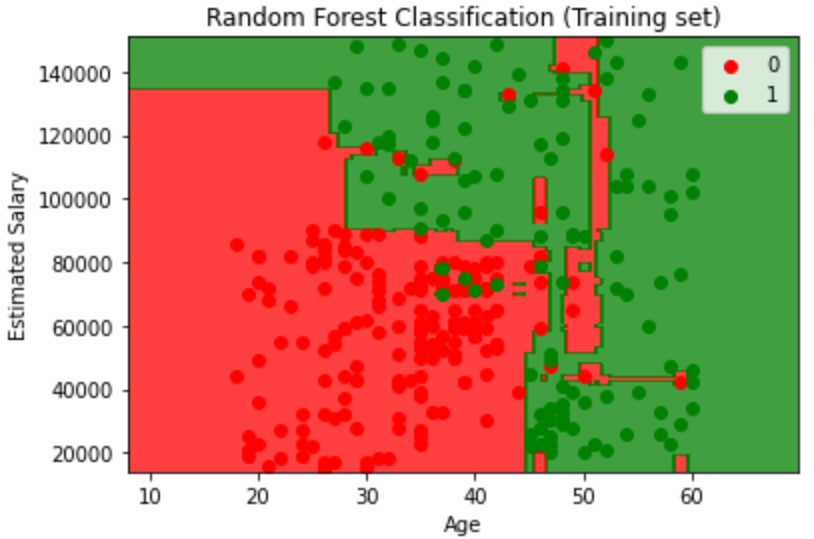
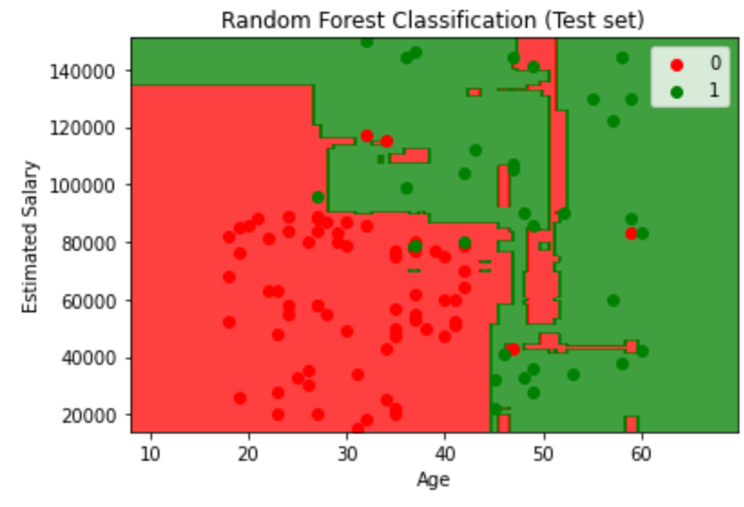
Training the Random Forest Classification model on the Training set

1
2
3

from sklearn.ensemble import RandomForestClassifier
classifier = RandomForestClassifier(n_estimators = 10, criterion = 'entropy', random_state = 0)
classifier.fit(X_train, y_train)

Making the Confusion Matrix

from sklearn.metrics import confusion_matrix, accuracy_score
cm = confusion_matrix(y_test, y_pred)
print(cm)
accuracy_score(y_test, y_pred)

1
2
3

[[63  5]
 [ 4 28]]
 0.91

Visualizing the Training set results

from matplotlib.colors import ListedColormap
X_set, y_set = sc.inverse_transform(X_train), y_train
X1, X2 = np.meshgrid(np.arange(start = X_set[:, 0].min() - 10,
								stop = X_set[:, 0].max() + 10, 
								step = 0.25),
                     np.arange(start = X_set[:, 1].min() - 1000,
                     			stop = X_set[:, 1].max() + 1000,
                                step = 0.25))
plt.contourf(X1, X2, 
classifier.predict(sc.transform(np.array([X1.ravel(), X2.ravel()]).T)).reshape(X1.shape),
             alpha = 0.75,
             cmap = ListedColormap(('red', 'green')))
plt.xlim(X1.min(), X1.max())
plt.ylim(X2.min(), X2.max())
for i, j in enumerate(np.unique(y_set)):
    plt.scatter(X_set[y_set == j, 0],
    			X_set[y_set == j, 1], 
    			c = ListedColormap(('red', 'green'))(i), 
    			label = j)
plt.title('Random Forest Classification (Training set)')
plt.xlabel('Age')
plt.ylabel('Estimated Salary')
plt.legend()
plt.show()

from matplotlib.colors import ListedColormap
X_set, y_set = sc.inverse_transform(X_test), y_test
X1, X2 = np.meshgrid(np.arange(start = X_set[:, 0].min() - 10, 
                               	stop = X_set[:, 0].max() + 10, 
                               	step = 0.25),
                     np.arange(start = X_set[:, 1].min() - 1000, 
                               stop = X_set[:, 1].max() + 1000,
                               step = 0.25))
plt.contourf(X1, X2, 
             classifier.predict(sc.transform(np.array([X1.ravel(), X2.ravel()]).T)).reshape(X1.shape),
             alpha = 0.75, 
             cmap = ListedColormap(('red', 'green')))
plt.xlim(X1.min(), X1.max())
plt.ylim(X2.min(), X2.max())
for i, j in enumerate(np.unique(y_set)):
    plt.scatter(X_set[y_set == j, 0],
                X_set[y_set == j, 1],
                c = ListedColormap(('red', 'green'))(i), 
                label = j)
plt.title('Random Forest Classification (Test set)')
plt.xlabel('Age')
plt.ylabel('Estimated Salary')
plt.legend()
plt.show()

随机森林可以用来进行体感游戏中对人体动作的检测，判断人生上的区域的运动等等。

https://www.microsoft.com/en-us/research/wp-content/uploads/2016/02/BodyPartRecognition.pdf