Hierarchical Clustering 层次聚类

原理

层次聚类的功能和K-Means 一样，也是将数据点进行聚类。有时候它们的结果是非常接近甚至完全相同的。

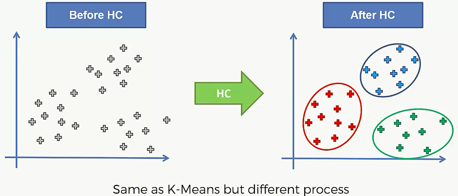
层次聚类分为： Agglomerative 和Divisive 两种。这篇博客要着重介绍的是 Agglomerative Hierarchical Clustering

一下是层次聚类的步骤:

Step1: Make each data point a single-point cluster :初始情况下，包含N个数据点的数据集就有N个类
Step2: Take the two closest data points and make them one cluster : 将距离最近的两个数据点合并成一个类，现在只有N-1个类了
Step3: Take the two closest clusters and make them one cluster :将两个距离最近的类合并成一个类，现在只有N-2个类了
Step4: 重复步骤3.直到只剩下一个类位置，得到最终聚类成果

现在很重要的一点是怎么来计算 cluster之间的距离？

在点和点之间我们可以用欧几里得距离，在两个类之间我们有4种不同的距离可以选择：

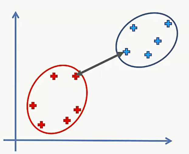
第一种：选择两个类中最近的点的距离

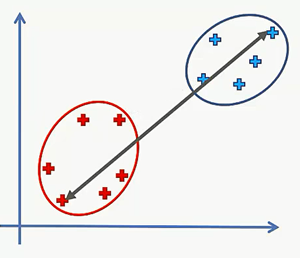
第二种：选择两个类中最远的点的距离

第三种：计算两个类中所有的点之间距离后取平均数

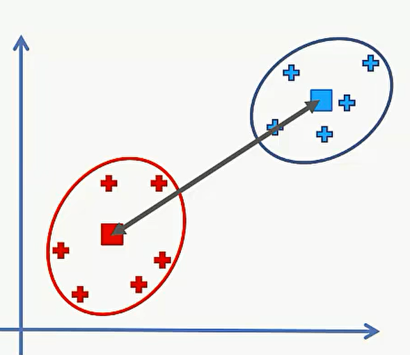
第四种：先计算两个类的中心点，然后求中心点之间的距离：

具体选择哪一种需要根据具体情况进行分析

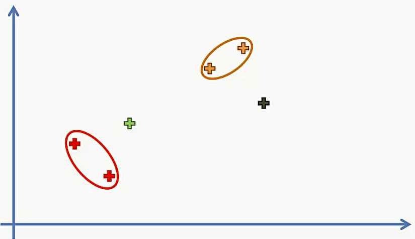
现在我们对一个具体的数据集进行简单的层级聚类：

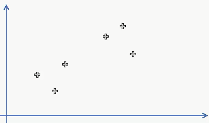
第一步，我们要将6个数据点分成6类：

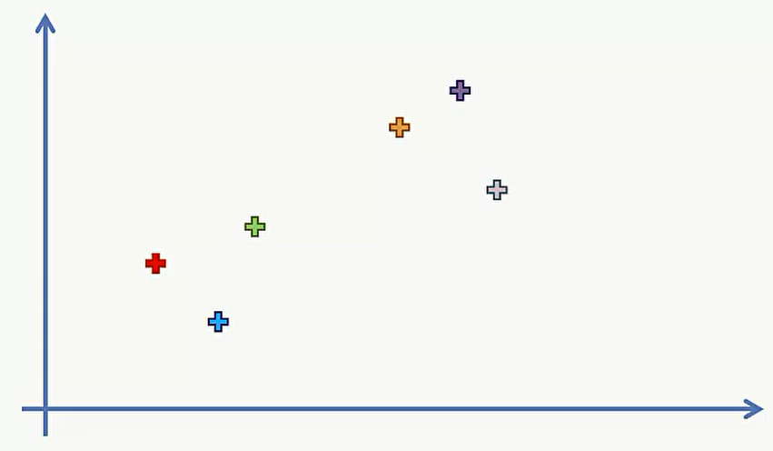
第二步，选择两个最近的点，合并成一个类，现在还有5个类：

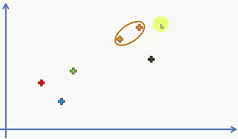
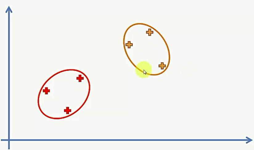
第三步，将两个最近的类合并成一个类，现在还有4 个类:

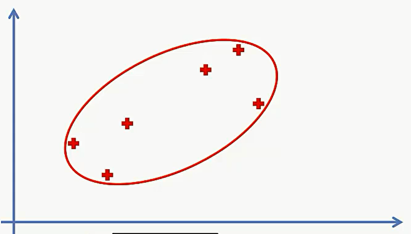
第四步，重复第三步直到只剩下一个类为止：

Dendrograms 树枝型结构联系图

我们可以用树枝型结构联系图来将聚类过程形象的表示出来。

如下图，左边是数据点的分布，右边是树枝型结构联系图。右图的x轴是离散的类，y轴是类与类之间的距离。

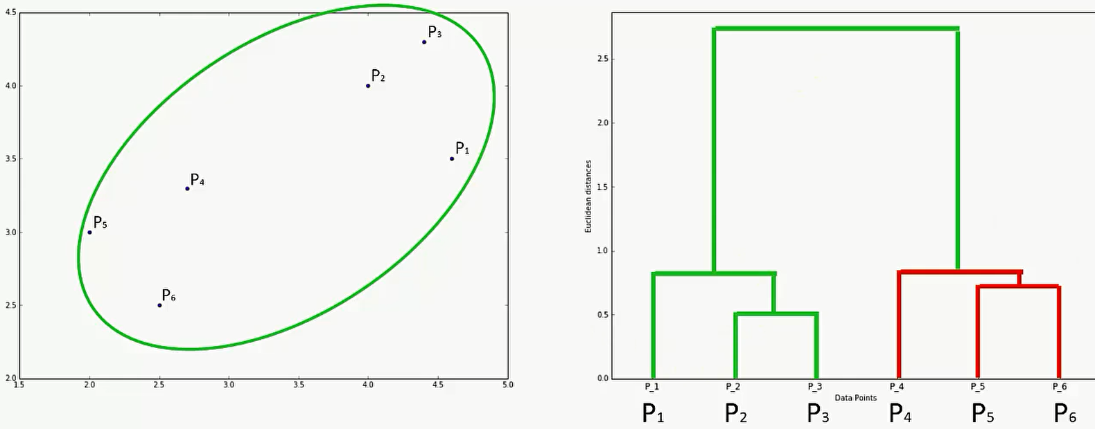
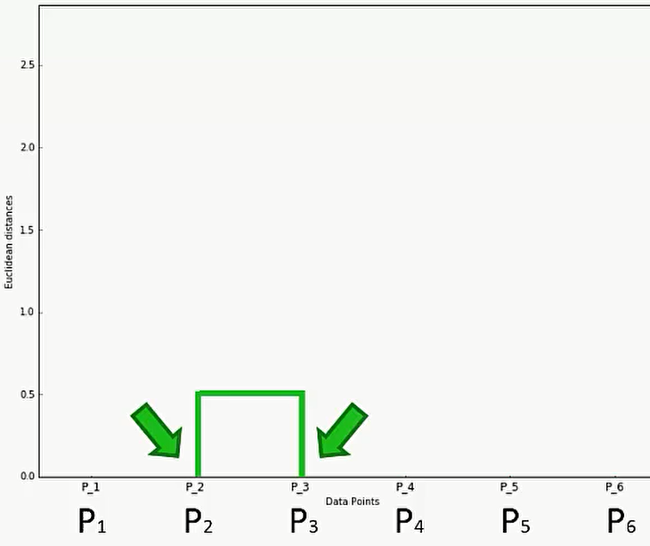
比如说首先是 P2和P3 是先聚合的，那么首先在P2和P3之间建立联系：

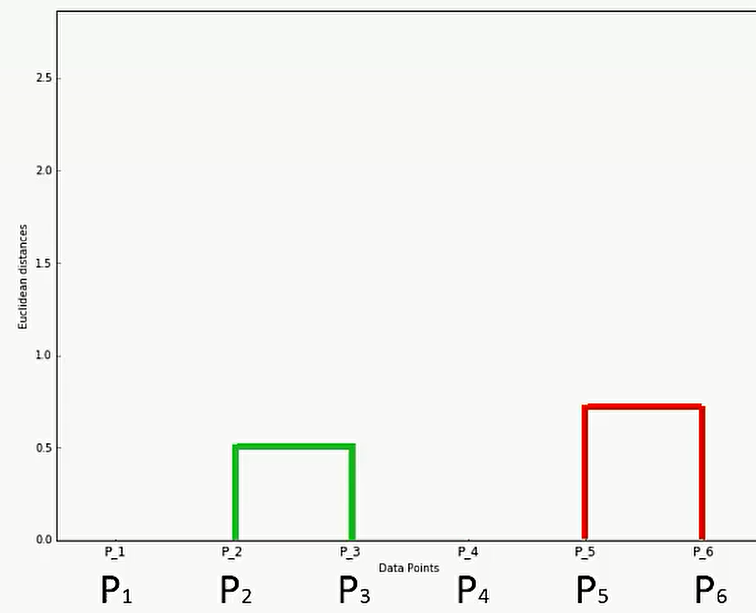
其次是在P5和P6之间进行联系，在图上可以这样反应：

那么我们怎么利用这个 Dengrograms？我们可以划分一个距离的最大值，高于这个距离的聚类就舍弃，低于这个距离的聚类就保留：

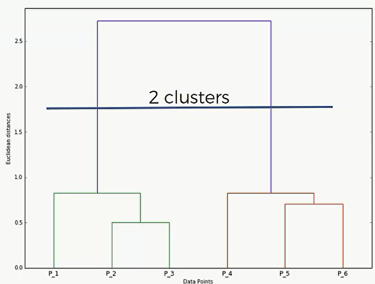
比如上图，我在1.75的地方画了一根线，那么就说明我们不要最终的那一类了，但是我们要保留1.75以下聚合的那两类。

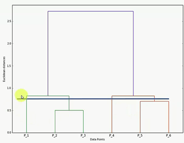
简单来说，只要看看这根线穿过了多少竖线，那么就说明分成几类。比如说下面，穿过了4根竖线，那么就说明分成4类

代码

我们用的数据集和K-Means数据集一样

Importing the libraries

1
2
3

import numpy as np
import matplotlib.pyplot as plt
import pandas as pd

Importing the dataset

1 2	dataset = pd.read_csv('Mall_Customers.csv') X = dataset.iloc[:, [3, 4]].values

Using the dendrogram to find the optimal number of clusters

import scipy.cluster.hierarchy as sch
dendrogram = sch.dendrogram(sch.linkage(X, method = 'ward'))
plt.title('Dendrogram')
plt.xlabel('Customers')
plt.ylabel('Euclidean distances')
plt.show()

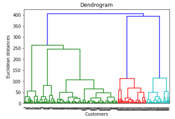
根据上图，我们可以看出选择3-5个 cluster是比较合适的

Training the Hierarchical Clustering model on the dataset

from sklearn.cluster import AgglomerativeClustering
hc = AgglomerativeClustering(n_clusters = 5, 
							affinity = 'euclidean',
                            linkage = 'ward')
y_hc = hc.fit_predict(X)

n_clusters 代表话分类的个数

affinity 是以什么关系来聚合，这里选的是欧氏距离

linkage 是指定的算法计算生成聚类树，有好几种取值方法，推荐使用 Ward

字符串	含义
single	最短距离（缺省）
complete	最大距离
average	平均距离
centroid	重心距离
ward	离差平方和方法（Ward方法）

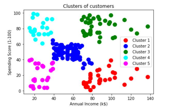
Visualising the clusters

plt.scatter(X[y_hc == 0, 0],
			X[y_hc == 0, 1],
            s = 100, 
            c = 'red', 
            label = 'Cluster 1')
plt.scatter(X[y_hc == 1, 0],
			X[y_hc == 1, 1],
            s = 100, c = 'blue',
            label = 'Cluster 2')
plt.scatter(X[y_hc == 2, 0],
			X[y_hc == 2, 1],
            s = 100, 
            c = 'green',
            label = 'Cluster 3')
plt.scatter(X[y_hc == 3, 0],
			X[y_hc == 3, 1],
            s = 100,
            c = 'cyan',
            label = 'Cluster 4')
plt.scatter(X[y_hc == 4, 0],
			X[y_hc == 4, 1],
            s = 100, 
            c = 'magenta', 
            label = 'Cluster 5')
plt.title('Clusters of customers')
plt.xlabel('Annual Income (k$)')
plt.ylabel('Spending Score (1-100)')
plt.legend()
plt.show()